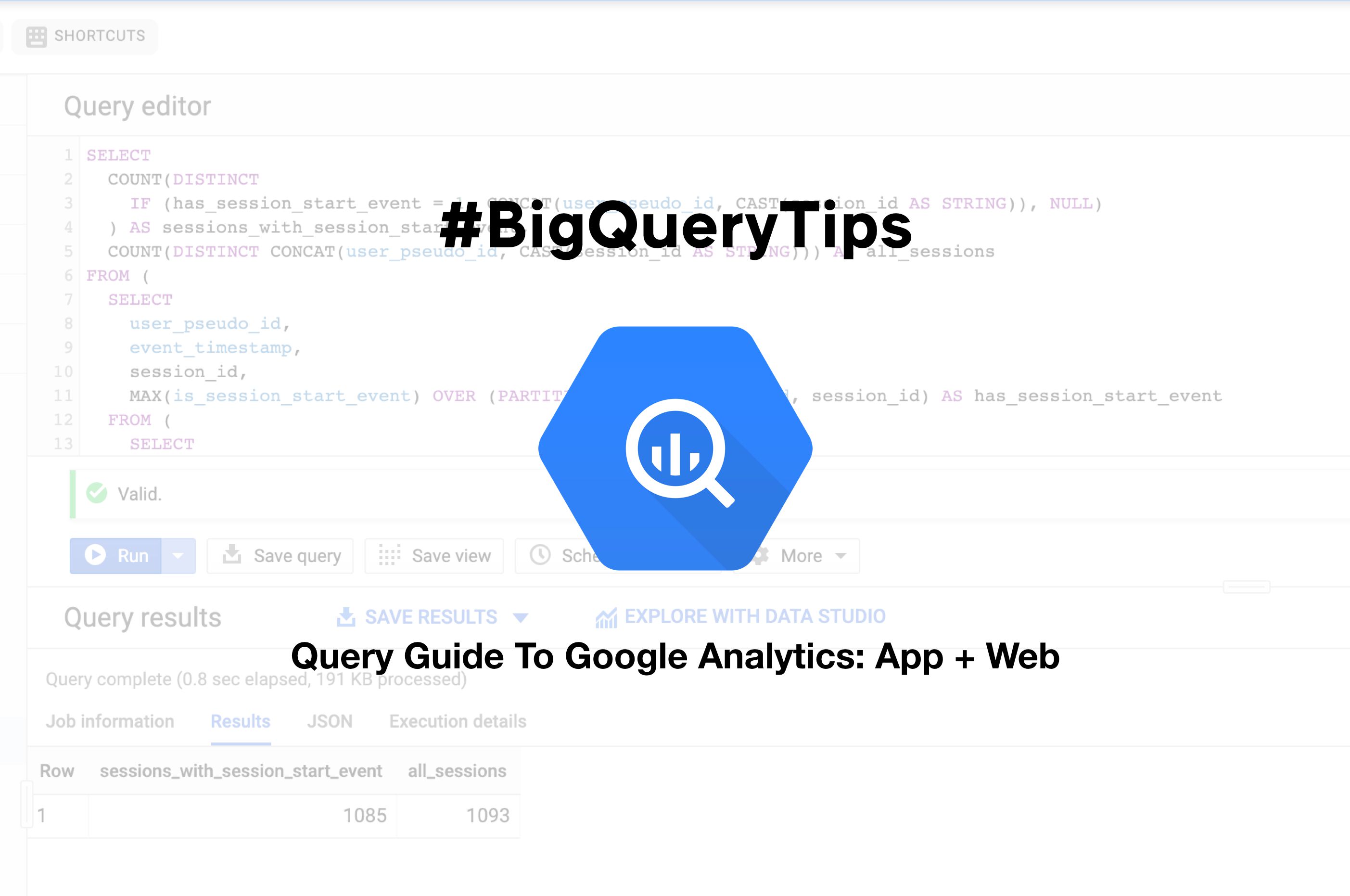
I’ve thoroughly enjoyed writing short (and sometimes a bit longer) bite-sized tips for my #GTMTips topic. With the advent of Google Analytics: App + Web and particularly the opportunity to access raw data through BigQuery, I thought it was a good time to get started on a new tip topic: #BigQueryTips.
For Universal Analytics, getting access to the BigQuery export with Google Analytics 360 has been one of the major selling points for the expensive platform. The hybrid approach of getting access to raw data that has nevertheless been annotated with Google Analytics’ sessionization schema and any integrations (e.g. Google Ads) the user might have enabled is a powerful thing indeed.
With Google Analytics: App + Web, the platform is moving away from the data model that has existed since the days of Urchin, and is instead converging with Firebase Analytics, to which we have already had access with native Android and iOS applications.
Fortunately, BigQuery export for App + Web properties comes at no additional platform costs - you only pay for storage and queries just as you would if creating a BigQuery project by yourself in Google’s cloud platform.
So, with data flowing into BigQuery, I thought it time to start writing about how to build queries against this columnar data store. One of the reasons is because I want to challenge myself, but the other reason is that there just isn’t that much information available online when it comes to using SQL with Firebase Analytics’ BigQuery exports.
To get things started with this new topic, I’ve enlisted the help of my favorite SQL wizard in #measure, Pawel Kapuscinski. He’s never short of a solution when tricky BigQuery questions pop up in Measure Slack, so I thought it would be great to get him to contribute with some of his favorite tips for how to approach querying BigQuery data with SQL.
Hopefully, #BigQueryTips will expand to more articles in the future. There certainly is a lot of ground to cover!
The Simmer Newsletter
Follow this link to subscribe to the Simmer Newsletter! Stay up-to-date with the latest content from Simo Ahava and the Simmer online course platform.
Getting started
First of all, you’ll naturally need a Google Analytics: App + Web property. Here are some guides for getting started:
- Step by Step: Setting up an App + Web Property (Krista Seiden)
- Getting Started With Google Analytics: App + Web (Simo)
- App + Web Properties tag and instrumentation guide (Google)
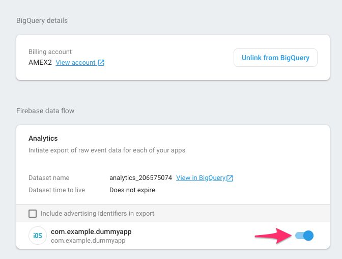
Next, you need to enable the BigQuery export for the new property, and for that you should follow this guide.
Once you have the export up-and-running, it’s a good time to take a moment to learn and/or get a refresher on how SQL works. For that, there is no other tutorial online that comes even close to the free, interactive SQL tutorial at Mode Analytics.
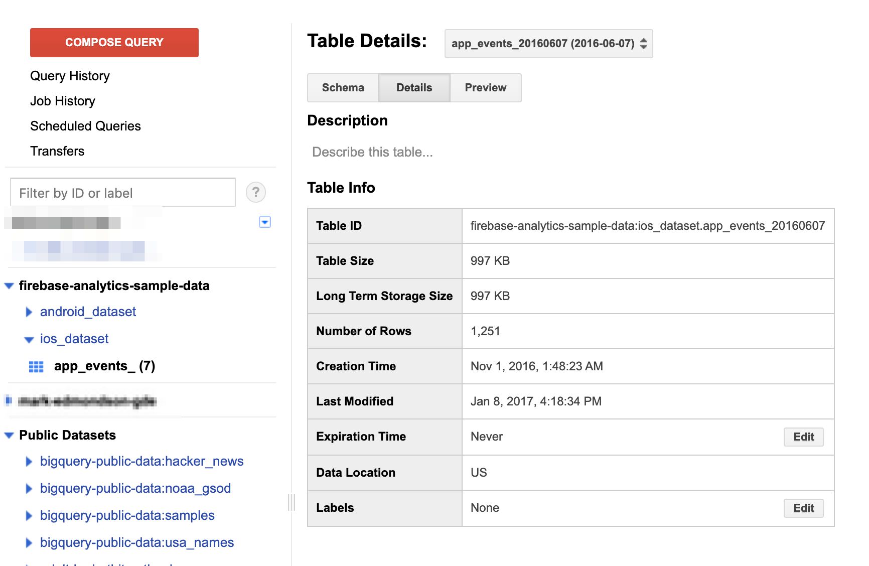
And once you’ve learned the difference between LEFT JOIN and CROSS JOIN, you can take a look at some of the sample data sets for iOS Firebase Analytics and Android Firebase Analytics. Play around with them, trying to figure out just how much querying a typical relational database differs from accessing data stored in columnar structure as BigQuery does.
At this point, you should have your BigQuery table collecting daily data dumps from the App + Web tags firing on your site, so let’s work with Pawel and introduce some pretty useful BigQuery SQL queries to get started on that data analysis path!
Tip #1: CASE and GROUP BY
Our first tip covers two extremely useful SQL statements: CASE and GROUP BY. Use these to aggregate and group your data!
CASE
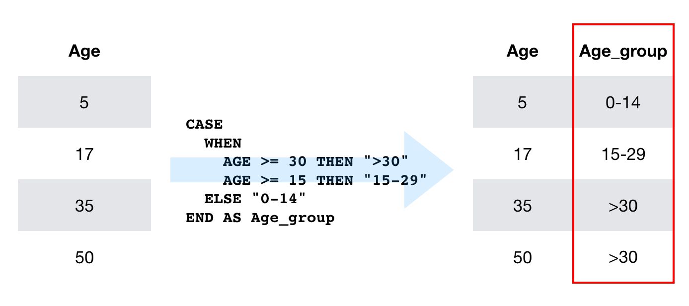
CASE statements are similar to the if...else statements used in other languages. The condition is introduced with the WHEN keyword, and the first WHEN condition that matches will have its THEN value returned as the value for that column.
You can use the ELSE keyword at the end to specify a default value. If ELSE is not defined and no conditions are met, the column gets the value null.
SOURCE TABLE
| user | age |
|---|---|
| 12345 | 15 |
| 23456 | 54 |
SQL
SELECT user, age,
  CASE
    WHEN age >= 90 THEN "90+"
    WHEN age >= 50 THEN "50-89"
    WHEN age >= 20 THEN "20-49"
    ELSE "0-19"
  END AS age_bucket
FROM some_table
QUERY RESULT
| user | age | age_bucket |
|---|---|---|
| 12345 | 15 | 0-19 |
| 23456 | 54 | 50-89 |
The CASE statement is useful for quick transformations and for aggregating the data based on simple conditions.
GROUP BY
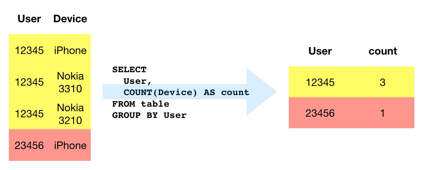
GROUP BY is required every time you want to summarize your data. For example, when you do calculations with COUNT (to return the number of instances) or SUM (to return the sum of instances), you need to indicate a column to group these calculations by (unless you’re only retrieving the calculated column) . GROUP BY is thus most often used with aggregate functions such as COUNT, MAX, ANY_VALUE, SUM, and AVG. It’s also used with some string functions such as STRING_AGG when aggregating multiple rows into a single string.
SOURCE TABLE
| user | mobile_device_model |
|---|---|
| 12345 | iPhone 5 |
| 12345 | Nokia 3310 |
| 23456 | iPhone 7 |
SQL
SELECT
  user,
  COUNT(mobile_device_model) AS device_count
FROM table
GROUP BY 1
QUERY RESULT
| user | device_count |
|---|---|
| 12345 | 2 |
| 23456 | 1 |
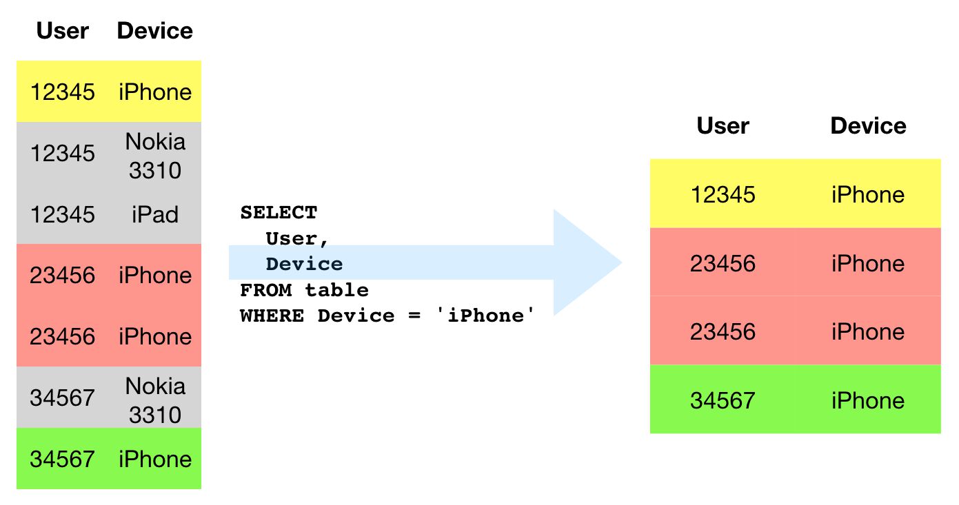
In the query above, we assume that a single user can have more than one device associated with them in the table that is being queried. As we do a COUNT of all the devices for a given user, we need to group the results by the user column for the query to work.
USE CASE: Device category distribution across users
Let’s keep the theme of users and devices alive for a moment.
Users and events are the key metrics for App + Web. This is fundamentally different to the session-centric approach of Google Analytics (even though there are reverberations of “sessions” in App + Web, too). It’s much closer to a true hit stream model than before.
However, event counts alone tell as nothing without us drilling into what kind of event happened.
In this first tip, we’ll learn to calculate the number of users per device category. As the concept of “User” is still bound to a unique browser client ID, if the same person visited the website on two different browser instances or devices, they would be counted as two users.
This is what the query looks like:
SELECT
  CASE
    WHEN device.category = "desktop" THEN "desktop"
    WHEN device.category = "tablet" AND app_info.id IS NULL THEN "tablet-web"
    WHEN device.category = "mobile" AND app_info.id IS NULL THEN "mobile-web"
    WHEN device.category = "tablet" AND app_info.id IS NOT NULL THEN "tablet-app"
    WHEN device.category = "mobile" AND app_info.id IS NOT NULL THEN "mobile-app"
  END AS device,
  COUNT(DISTINCT user_pseudo_id) AS users
FROM
  `dataset.analytics_accountId.events_2*`
GROUP BY
  1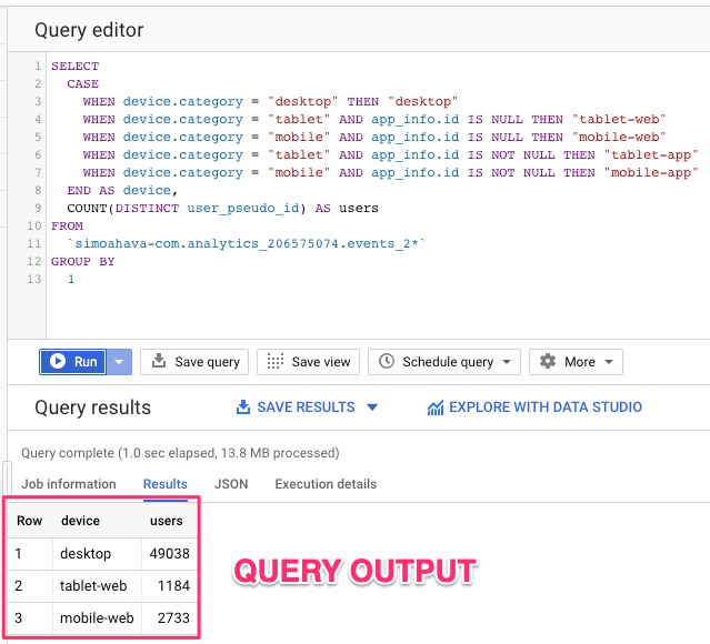
The query itself is simple, but it makes use of the two statements covered in this chapter effectively. CASE is used to segment “mobile” and “tablet” users further into web and app groups (something you’ll find useful once you start collecting data from both websites and mobile apps), and GROUP BY displays the count of unique device IDs per device category.
Tip #2: DISTINCT and HAVING
The next two keywords we’ll cover are HAVING and DISTINCT. The first is great for filtering results based on aggregated values. The latter is used to deduplicate results to avoid calculating the same result multiple times.
DISTINCT
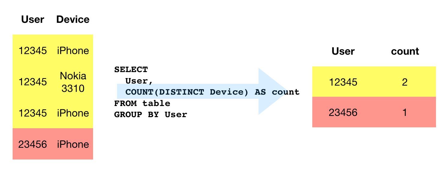
The DISTINCT keyword is used to deduplicate results.
SOURCE TABLE
| user | device_category | session_id |
|---|---|---|
| 12345 | desktop | abc123 |
| 12345 | desktop | def234 |
| 12345 | tablet | efg345 |
| 23456 | mobile | fgh456 |
SQL
SELECT
  user,
  COUNT(DISTINCT device_category) AS device_category_count
FROM
  table
GROUP BY
  1
QUERY RESULT
| user | device_category_count |
|---|---|
| 12345 | 2 |
| 23456 | 1 |
For example, if the user had three sessions with device categories desktop, desktop, and tablet, then a query for COUNT(DISTINCT device.category) would return 2, as there are just two instances of distinct device categories.
HAVING
The HAVING clause can be used at the end of the query, after all calculations have been done, to filter the results. All the rows selected for the query are still processed, even if the HAVING statement strips out some of them from the result table.
SOURCE TABLE
| user | device_category | session_id |
|---|---|---|
| 12345 | desktop | abc123 |
| 12345 | desktop | def234 |
| 12345 | tablet | efg345 |
| 23456 | mobile | fgh456 |
SQL
SELECT
  user,
  COUNT(DISTINCT device_category) AS device_category_count
FROM
  table
GROUP BY
  1
HAVING
  device_category_count > 1
QUERY RESULT
| user | device_category_count |
|---|---|
| 12345 | 2 |
It’s similar to WHERE (see next chapter), but unlike WHERE which is used to filter the actual records that are processed by the query, HAVING is used to filter on aggregated values. In the query above, device_category_count is an aggregated count of all the distinct device categories found in the data set.
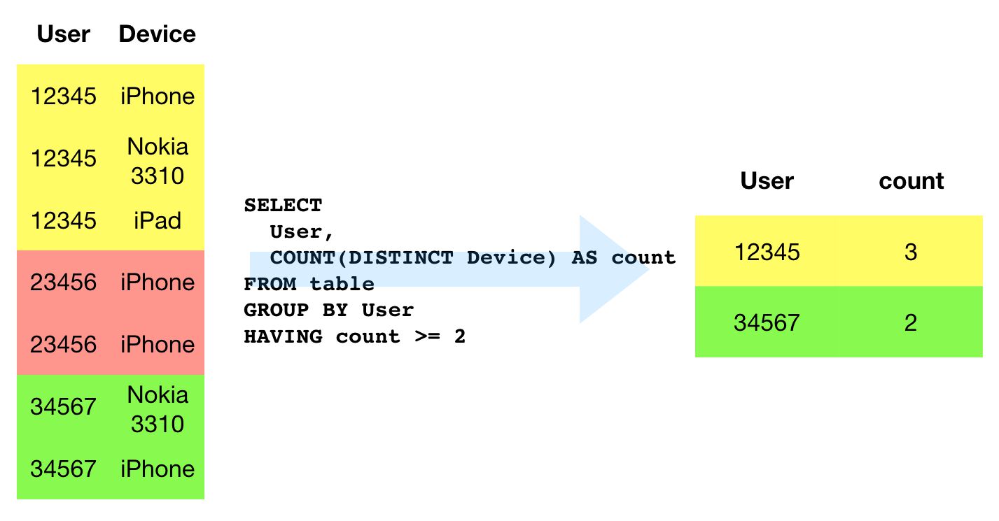
USE CASE: Distinct device categories per user
Since the very name, App + Web, implies cross-device measurement, exploring some ways of grouping and filtering data based on users with more than one device in use seems fruitful.
The query is similar to the one in the previous chapter, but this time instead of grouping by device category, we’re grouping by user and counting the number of unique device categories each user has visited the site with. We’re filtering the data to only include users with more than one device category in the data set.
This is an exploratory query. You can then extend it to actually detect different models instead of just using device category. Device category is a fickle dimension to use, as in the example dataset used for this article, many times a device labelled as “Apple iPhone” was actually counted as a Desktop device.
See this article by Craig Sullivan to understand how messed up device attribution in web analytics actually is.
SELECT
  user_pseudo_id,
  COUNT(DISTINCT device.category) AS used_devices_count,
  STRING_AGG(DISTINCT device.category) AS distinct_devices,
  STRING_AGG(device.category) AS devices
FROM
  `dataset.analytics_accountId.events_2*`
GROUP BY
  1
HAVING
  used_devices_count > 1
As a bonus, you can see how STRING_AGG can be used to concatenate multiple values into a single column. This is useful for identifying patterns that emerge across multiple rows of data!
Tip #3: WHERE
WHERE
If you want to filter the records against which you’ll run your query, WHERE is your best friend. As it filters the records that are processed, it’s also a great way to reduce the (performance and monetary) cost of your queries.
SOURCE TABLE
| user | session_id | landing_page_path |
|---|---|---|
| 12345 | abc123 | /home/ |
| 12345 | bcd234 | /purchase/ |
| 23456 | cde345 | /home/ |
| 34567 | def456 | /contact-us/ |
SQL
SELECT
  *
FROM
  table
WHERE
  user = '12345'
QUERY RESULT
| user | session_id | landing_page_path |
|---|---|---|
| 12345 | abc123 | /home/ |
| 12345 | bcd234 | /purchase/ |
The WHERE clause is used to filter the rows against which the rest of the query is made. It is introduced directly after the FROM statement, and it reads as “return all the rows in the FROM table that match the condition of the WHERE clause”.
Do note that WHERE can’t be used with aggregate values. So if you’ve done any calculations with the rows returned from the table, you need to use HAVING instead.
Due to this, WHERE is less expensive in terms of query processing than HAVING.
USE CASE: Engaged users
As mentioned before, App + Web is event-driven. With Firebase Analytics, Google introduced a number of automatically collected, pre-defined events to help users gather useful data from their apps and websites without having to flex a single muscle.
One such event is user_engagement. This is fired when the user has engaged with the website or app for a specified period of time.
Since this is readily available as a custom event, we can create a simple query that uses the WHERE clause to return only those records where the user was engaged.
The key to WHERE is that it’s executed after the FROM clause (which specifies the table to be queried). If a row doesn’t match the condition in WHERE, it won’t be used to match the rest of the query against.
SELECT
  event_date,
  COUNT(DISTINCT user_pseudo_id) AS engaged_users
FROM
  `dataset.analytics_accountId.events_20190922`
WHERE
  event_name = "user_engagement"
GROUP BY
  1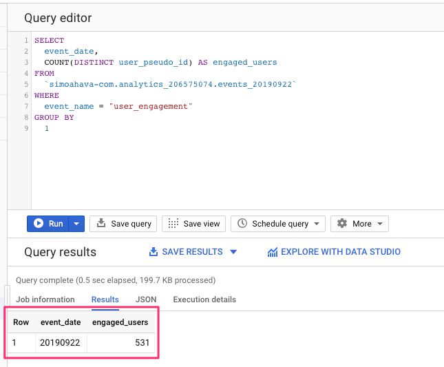
See how we’re including data from just one date? We’re also only including DISTINCT users, so if a user was engaged more than once during the day we’re only counting them once.
Tip #4: SUBQUERIES and ANALYTIC functions
A subquery in SQL means a query within a query. They can emerge in multiple different places, such as within SELECT clauses, FROM clauses, and WHERE clauses.
Analytic functions let you do calculations that cover other rows than just the one that is being processed. It’s similar to aggregations such as SUM and AVG except it doesn’t result in rows getting grouped into a single result. That’s why analytic functions are perfectly suited for things like running totals/averages or, in analytics contexts, determining session boundaries by looking at first and last timestamps, for example.
SUBQUERY
The point of a subquery is to run calculations on table data, and return the result of those calculations to the enclosing query. This lets you logically organize your queries, and it makes it possible to do calculations on calculations, which would not be possible in a single query.
SOURCE TABLE
| user | event_name |
|---|---|
| 12345 | session_start |
| 23456 | user_engagement |
| 34567 | user_engagement |
| 45678 | link_click |
SQL
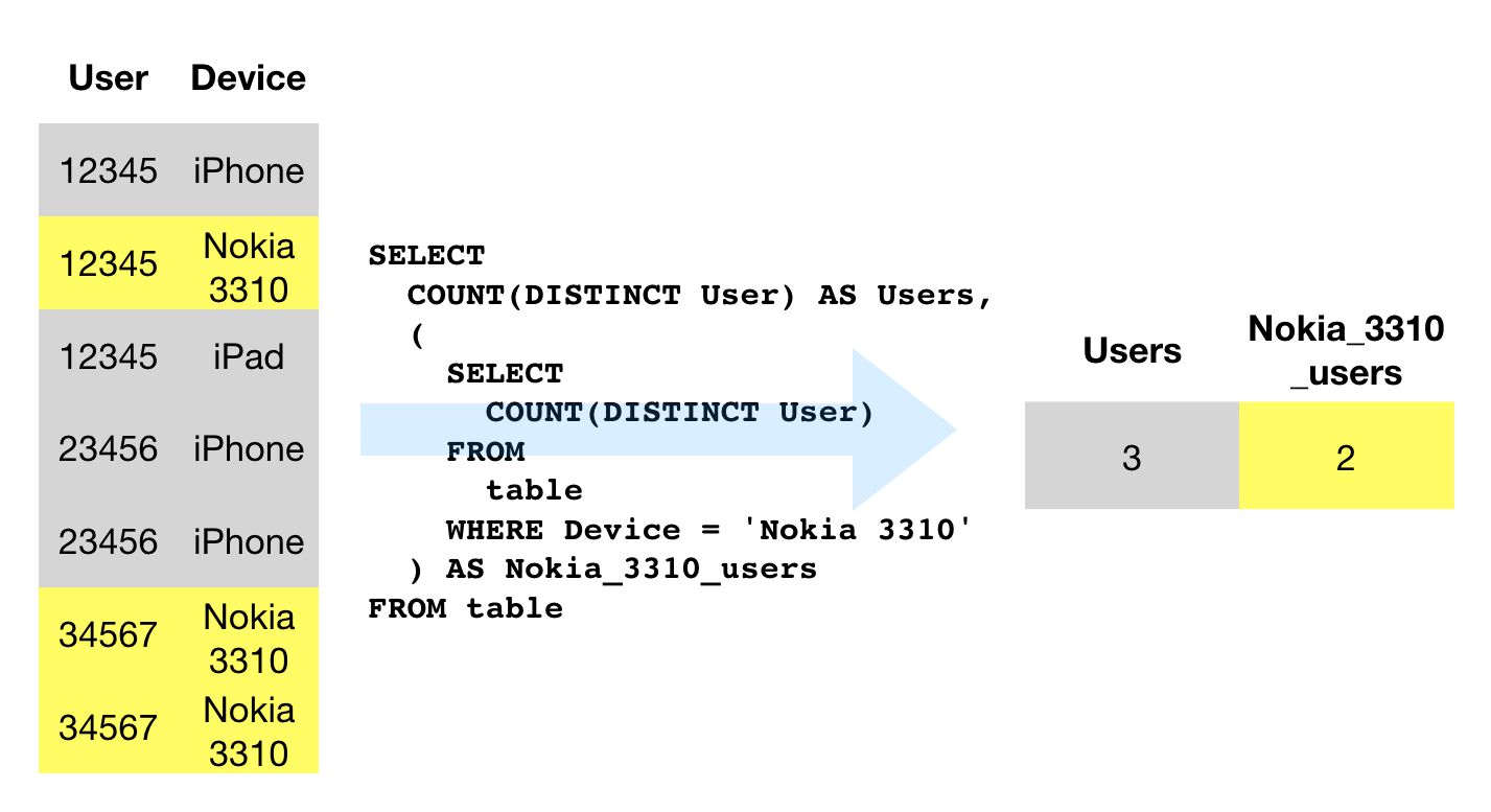
SELECT
  COUNT(DISTINCT user) AS all_users,
  (
    SELECT
      COUNT(DISTINCT user)
    FROM
      table
    WHERE
      event_name = 'user_engagement'
  ) AS engaged_users
FROM
  table
QUERY RESULT
| all_users | engaged_users |
|---|---|
| 4 | 2 |
In this example, the subquery is within the SELECT statement, meaning the subquery result is bundled into a single column of the main query.
Here, the engaged_users column retrieves the count of all distinct user IDs from the table, where these users had an event named user_engagement collected at any time.
The main query then combines this with a count of all distinct user IDs without any restrictions, and thus you get both counts in the same table.
You couldn’t have achieved with just the main query, since the WHERE statement applies to all SELECT columns in the table. That’s why we needed the subquery - we had to use a WHERE statement that only applied to the engaged_users column.
ANALYTIC FUNCTIONS
Analytic functions can be really difficult to understand, since with SQL you’re used to going over the table row-by-row, and comparing the query against each row one at a time.
With an analytic function, you stretch this logic a bit. The query still goes over the source table row-by-row, but this time you can reference other rows when doing calculations.
SOURCE TABLE
| user | event_name | event_timestamp |
|---|---|---|
| 12345 | click | 1001 |
| 12345 | click | 1002 |
| 23456 | session_start | 1012 |
| 23456 | user_engagement | 1009 |
| 34567 | click | 1000 |
SQL
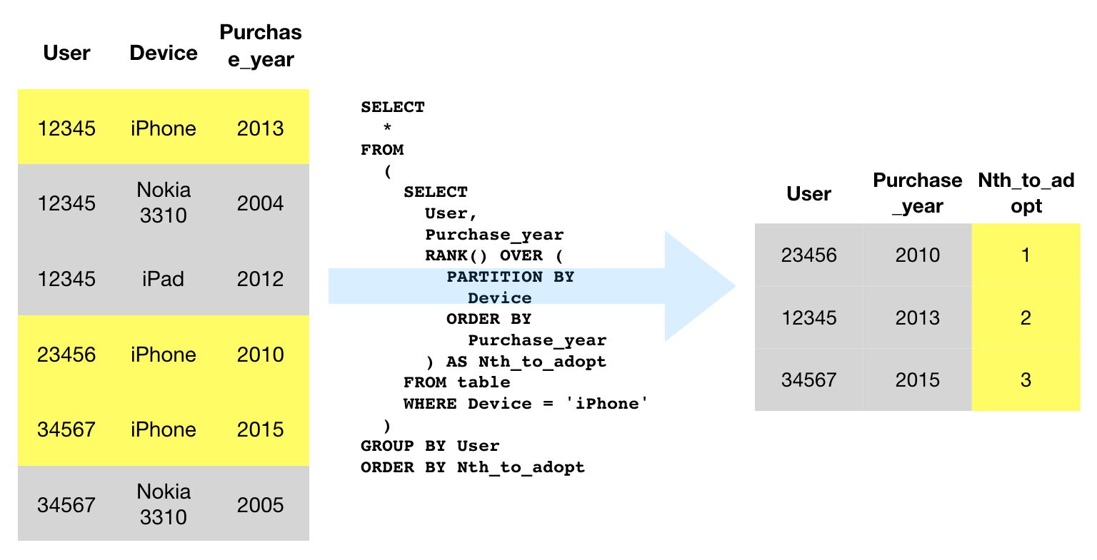
SELECT
  event_name,
  user,
  event_timestamp
FROM (
  SELECT
    user,
    event_name,
    event_timestamp,
    RANK() OVER (PARTITION BY event_name ORDER BY event_timestamp) AS rank
  FROM
    table
)
WHERE
  rank = 1
QUERY RESULT
| event_name | user | event_timestamp |
|---|---|---|
| click | 34567 | 1000 |
| user_engagement | 23456 | 1009 |
| session_start | 23456 | 1012 |
In this query, we take each event and see which user sent the first such event in the table.
For each row in the table, the RANK() OVER (PARTITION BY event_name ORDER BY event_timestamp) AS rank is run. The partition is basically a “reference” table with all the event names matching the current row’s event name, and their respective timestamps.
These timestamps are then ordered in ascending order (within the partition). The RANK() OVER part of the function returns the current event name’s rank in this table.
To walk through an example, let’s say the query engine encounters the first row of the table. The RANK() OVER (PARTITION BY event_name ORDER BY event_timestamp) creates the reference table that looks like this for the first row:
| user | event_name | event_timestamp | rank |
|---|---|---|---|
| 12345 | click | 1000 | 1 |
| 12345 | click | 1001 | 2 |
| 12345 | click | 1002 | 3 |
The query then checks how the current row matches against this partition, and returns 2 as the first row in the table was rank 2 of its partition.
This partition is ephemeral - it’s only used to calculate the result of the analytic function.
For the purposes of this exercise, this analytic function is furthermore done in a subquery, so that the main query can filter the result using a WHERE for just those items that had rank 1 (first timestamp of any given event).
I recommend checking out the first paragraphs in this document - it explains how the partitioning works.
USE CASE: First interaction per event
Let’s extend the example from above into the App + Web dataset.
We’ll create a list of client IDs together with the event name, the timestamp, and the timestamp converted to a readable (date) format.
SELECT
  user_pseudo_id,
  event_name,
  event_timestamp,
  DATETIME(TIMESTAMP_MICROS(event_timestamp), "Europe/Helsinki") AS date
FROM (
  SELECT
    user_pseudo_id,
    event_name,
    event_timestamp,
    RANK() OVER (PARTITION BY event_name ORDER BY event_timestamp) AS rank
  FROM
    `dataset.analytics_accountId.events_20190922` )
WHERE
  rank = 1
ORDER BY
  event_timestamp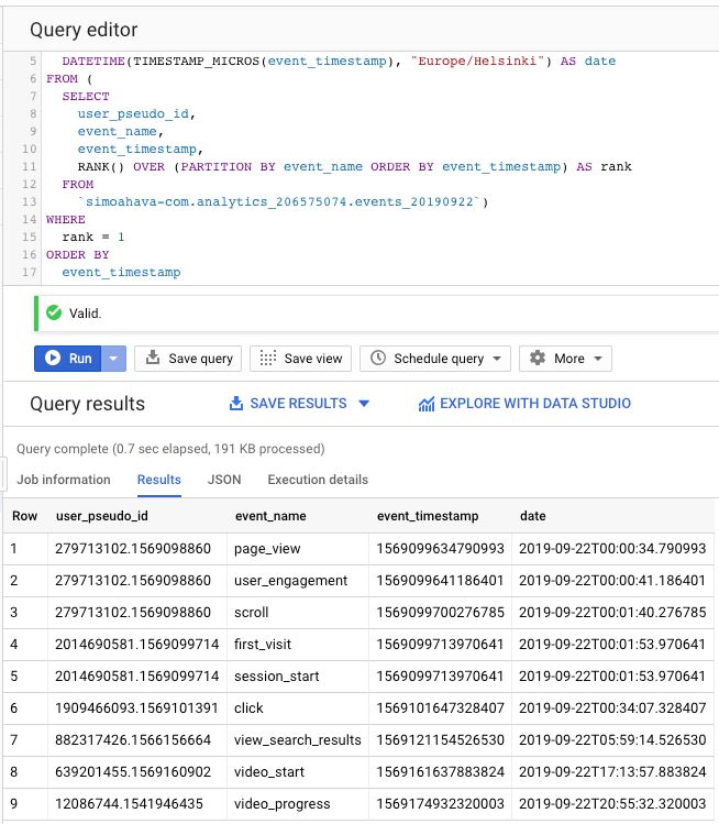
The logic is exactly the same as in the introduction to analytic functions above. The only difference is how we use the DATETIME and TIMESTAMP_MICROS to turn the UNIX timestamp (stored in BigQuery) into a readable date format.
Don’t worry - analytic functions in particular are a tough concept to understand. Play around with the different analytic functions to get an idea of how they work with the source idea.
There are quite a few articles and videos online that explain the concept further, so I recommend checking out the web for more information. We will also return to analytic functions many, many times in future #BigQueryTips posts.
Tip #5: UNNEST and CROSS JOIN
The dataset exported by App + Web does not end up in a relational database where we could use the JOIN key to quickly pull in extra information about pages, sessions, and users.
Instead, BigQuery arranges data in nested and repeated fields - that’s how it can have a single row represent all the hits of a session (as in the Google Analytics dataset).
The problem with this approach is that it’s not too intuitive to access these nested values.
Enter UNNEST, particularly when coupled with CROSS JOIN.
UNNEST means that the nested structure is actually expanded so that each item within can be joined with the rest of the columns in the row. This results in the single row becoming multiple rows, where each row corresponds to one value in the nested structure. This column-to-rows is achieved with a CROSS JOIN, where every item in the unnested structure is joined with each column in the rest of the table.
UNNEST and CROSS JOIN
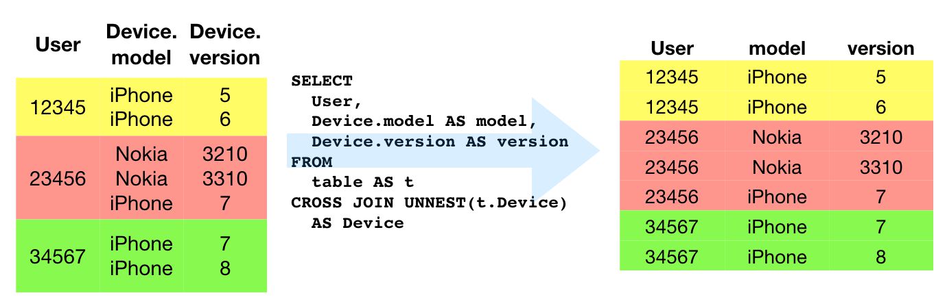
The two keywords go intrinsically together, so we’ll treat them as such.
SOURCE TABLE
| timestamp | event | params.key | params.value |
|---|---|---|---|
| 1000 | click | time type device | 10 right-click iPhone |
SQL
SELECT
  timestamp,
  event,
  event_params.key AS event_params_key
FROM
  table AS t
  CROSS JOIN UNNEST (t.params) AS event_params
QUERY RESULT
| timestamp | event | event_params_key |
|---|---|---|
| 1000 | click | time |
| 1000 | click | type |
| 1000 | click | device |
See what happened? The nested structure within params was unnested so that each item was treated as a separate row in its own column. Then, this unnested structure was cross-joined with the table. A CROSS JOIN combines every row from table with every row from the unnested structure.
This is how you end up with a structure that you can then use for calculations in your main query.
It’s a bit complicated since you always need to do the UNNEST - CROSS JOIN exercise, but once you’ve done it a few times it should become second nature.
In fact, there’s a shorthand for writing the CROSS JOIN that might make things easier to read (or not). You can replace the CROSS JOIN statement with a comma. This is what the example query would look like when thus modified.
SELECT
  timestamp,
  event,
  event_params.key AS event_params_key
FROM
  table AS t,
  UNNEST (t.params) AS event_params
USE CASE: Pageviews and Unique Pageviews per user
Let’s look at a query for getting the count of pageviews and unique pageviews per user.
SELECT
  event_date,
  event_params.value.string_value as page_url,
  COUNT(*) AS pageviews,
  COUNT(DISTINCT user_pseudo_id) AS unique_pageviews
FROM
  `dataset.analytics_accountId.events_20190922` AS t,
  UNNEST(t.event_params) AS event_params
WHERE
  event_params.key = "page_location"
  AND event_name = "page_view"
GROUP BY
  1,
  2
ORDER BY
  3 DESC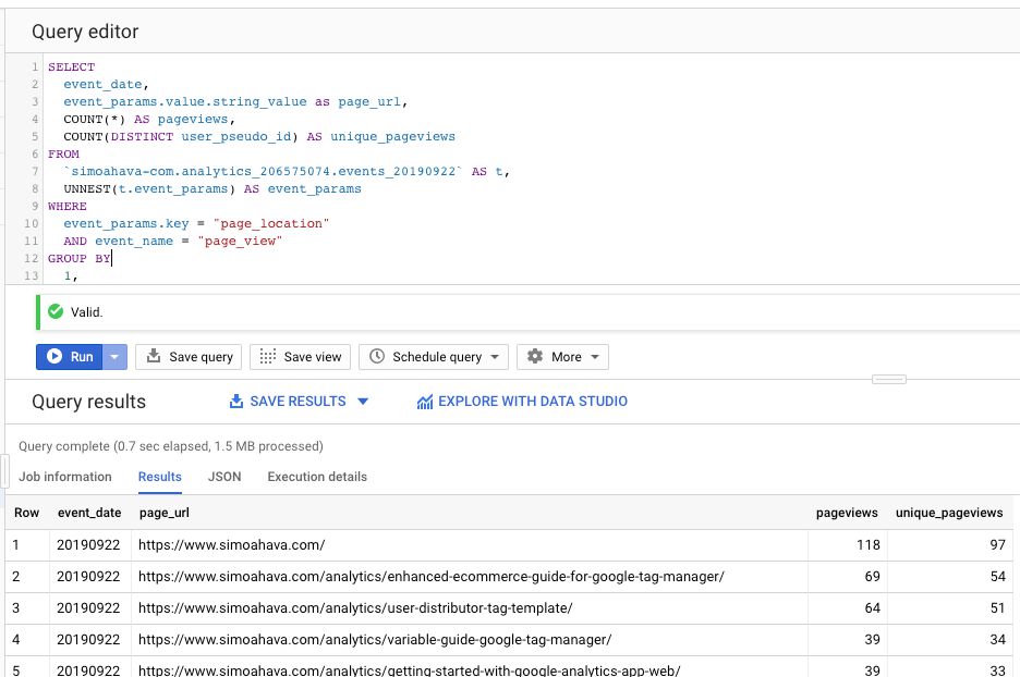
In the FROM statement we define the table as usual, and we give it an alias t (good practice, as it helps keep the queries lean).
The next step is to UNNEST one of those nested fields, and then CROSS JOIN it with the rest of our table. The WHERE clause is used to make sure only rows that have the page_location key and the page_view event type are included in the final table.
Finally, we GROUP BY the event date and page URL, and then we sort everything by the count of pageviews in descending order.
Conceptually, the UNNEST and CROSS JOIN create a new table that has a crazy number of rows, as every row in the original table is multiplied by the number of rows in the event_params nested structure. The WHERE clause is thus your friend in making sure you only analyze the data that answers the question you have.
Tip #6: WITH…AS and LEFT JOIN
The final keywords we’ll go through are WITH...AS and LEFT JOIN. The first lets you create a type of subquery that you can reference in your other queries as a separate table. The second lets you join two datasets together while preserving rows that do not match against the join condition.
WITH…AS
WITH...AS is very similar conceptually to a subquery. It allows you to build a table expression that can then be used by your queries. The main difference to a subquery is that the table gets an alias, and you can then use this alias wherever you want to refer to the table’s data. A subquery would need to be repeated in all places where you want to reference it, so WITH makes custom queries more accessible.
SOURCE TABLE
| user | event_name | event_timestamp |
|---|---|---|
| 12345 | click | 1000 |
| 12345 | user_engagement | 1005 |
| 12345 | click | 1006 |
| 23456 | session_start | 1002 |
| 34567 | session_start | 1000 |
| 34567 | click | 1002 |
SQL
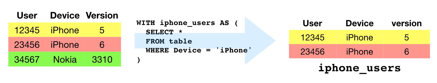
WITH users_who_clicked AS (
  SELECT
    DISTINCT user
  FROM
    table
  WHERE event_name = 'click'
)
SELECT
  *
FROM
  users_who_clicked
QUERY RESULT
| user |
|---|
| 12345 |
| 34567 |
It’s not the most mind-blowing of examples, but it should illustrate how to use table aliases. After the WITH...AS clause, you can then reference the table in e.g. FROM statements and in joins.
See the next example where we make this more interesting.
LEFT JOIN
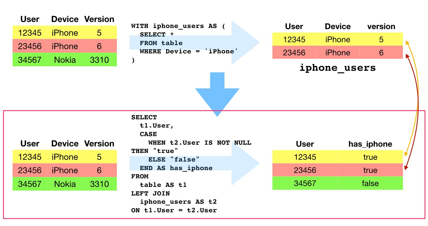
A LEFT JOIN is one of the most useful data joins because it allows you to account for unmatched rows as well.
A LEFT JOIN takes all rows in the first table (“left” table), and the rows that match a specific join criterion in the second table (“right” table). For all the rows that did not have a match, the first table is populated with a null value. Rows in the second table that do not have a match in the first table are discarded.
SOURCE TABLE
| user | event_name | event_timestamp |
|---|---|---|
| 12345 | click | 1000 |
| 12345 | user_engagement | 1005 |
| 12345 | click | 1006 |
| 23456 | session_start | 1002 |
| 34567 | session_start | 1000 |
| 34567 | click | 1002 |
SQL
WITH users_who_clicked AS (
  SELECT
    DISTINCT user
  FROM
    table
  WHERE event_name = 'click'
)
SELECT
  t1.user,
  CASE
    WHEN t2.user IS NOT NULL THEN "true"
    ELSE "false"
  END AS user_did_click
FROM
  table as t1
LEFT JOIN
  users_who_clicked as t2
ON
  t1.user = t2.user
GROUP BY
  1, 2
QUERY RESULT
| user | user_did_click |
|---|---|
| 12345 | true |
| 23456 | false |
| 34567 | true |
With the LEFT JOIN, we take all the user IDs in the main table, and then we take all the rows in the users_who_clicked table (that we created in the WITH...AS tutorial above). For all the rows where the user ID from the main table has a match in the users_who_clicked table, we populate a new column named user_did_click with the value true.
For all the user IDs that do not have a match in the users_who_clicked table, the value false is used instead.
USE CASE: Simple segmenting
Let’s put a bunch of things we’ve now learned together, and replicate some simple segmenting functionality from Google Analytics in BigQuery.
WITH
  engaged_users_table AS (
  SELECT
    DISTINCT event_date,
    user_pseudo_id
  FROM
    `dataset.analytics_accountId.events_20190922`
  WHERE
    EVENT_NAME = "user_engagement"),
  pageviews_table AS (
  SELECT
    DISTINCT event_date,
    event_params.value.string_value AS page_url,
    user_pseudo_id
  FROM
    `simoahava-com.analytics_206575074.events_20190922` AS t,
    UNNEST(t.event_params) AS event_params
  WHERE
    event_params.key = "page_location"
    AND event_name = "page_view")
SELECT
  t1.event_date,
  page_url,
  COUNTIF(t2.user_pseudo_id IS NOT NULL) AS engaged_users_visited,
  COUNTIF(t2.user_pseudo_id IS NULL) AS not_engaged_users_visited
FROM
  pageviews_table AS t1
LEFT JOIN
  engaged_users_table AS t2
ON
  t1.user_pseudo_id = t2.user_pseudo_id
GROUP BY
  1,
  2
ORDER BY
  3 DESC
Let’s chop this down to pieces again.
In the query above, we have two table aliases created. The first one named engaged_users_table should be familiar - it’s the query we built in tip #3.
The second one named pageviews_table should ring a bell as well. We built it in tip #5.
We create these as table aliases so that we can use them in the subsequent join.
Now, let’s look at the rest of the query:
SELECT
  t1.event_date,
  page_url,
  COUNTIF(t2.user_pseudo_id IS NOT NULL) AS engaged_users_visited,
  COUNTIF(t2.user_pseudo_id IS NULL) AS not_engaged_users_visited
FROM
  pageviews_table AS t1
LEFT JOIN
  engaged_users_table AS t2
ON
  t1.user_pseudo_id = t2.user_pseudo_id
GROUP BY
  1,
  2
ORDER BY
  3 DESC
Focus on the part after the FROM clause. Here, we take the two tables, and we LEFT JOIN them. The pageviews_table is the “left” table, and engaged_users is the “right” table.
LEFT JOIN takes all the rows in the “left” table and the matching rows from the “right” table. The matching criterion is established in the ON clause. Thus, a match is made if the user_pseudo_id is the same between the two tables.
To illustrate, this is what a simple LEFT JOIN without any calculations or aggregations would look like:
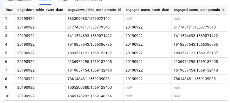
Here you can see that on rows 1, 9, and 10 there was no match for the user_pseudo_id in the engaged_users table. This means that the user who dispatched this pageview was not considered “engaged” in the date range selected for analysis.
If you’re wondering what COUNTIF does, then check out these two statements detail:
COUNTIF(
  t2.user_pseudo_id IS NOT NULL
) AS engaged_users_visited,

COUNTIF(
  t2.user_pseudo_id IS NULL
) AS not_engaged_users_visited
The first one increments the engaged_users_visited counter by one for all the rows where the user visited the page AND had a row in the engaged_users table.
The second one increments the not_engaged_users_visited counter by one for all the rows where the user visited the page and DID NOT have a row in the engaged_users table.
We can do this because the LEFT JOIN leaves the t2.* columns null in case the user ID from the pageviews_table was not found in the engaged_users_table.
SUMMARY
Phew!
That wasn’t a quick foray into BigQuery after all.
However, if you already possess a rudimentary understanding of SQL (and if you don’t, just take a look at the Mode Analytics tutorial), then the most complex things you need to wrap your head around are the ways in which BigQuery leverages its unique columnar format.
It’s quite different to a relational database, where joins are the most powerful tool in your kit for running analyses against different data structure.
In BigQuery, you need to understand the nested structures and how to UNNEST them. This, for many, is a difficult concept to grasp, but once you consider how UNNEST and CROSS JOIN simply populate the table as if it had been a flat structure all along, it should help you build the queries you want.
Analytic functions are arguably the coolest thing since Arnold Schwarzenegger played Mr. Freeze. They let you do aggregations and calculations without having to build a complicated mess of subqueries across all the rows you want to process. We’ve only explored a very simple use case here, but in subsequent articles we’ll definitely cover these in more detail.
Finally, huge thanks to Pawel for providing the SQL examples and walkthroughs. Simo contributed some enhancements to the queries, but his contribution is mainly editorial. Thus, direct all criticism and suggestions for improvement to him, and him alone.
If you’re an analyst working with Google Analytics and thinking about what you should do to improve your skill set, we recommend learning SQL and then going to town on either any one of the copious BigQuery sample datasets out there, or on your very own App + Web export.
Let us know in the comments if questions arose from this guide!